Sentiment Analysis of Amazon Reviews
In this mini-project, I explore different methods for analyzing the sentiment of Amazon product reviews. I employ a dataset containing the text of product reviews and corresponding product ratings assigned by each reviewer. I compare the predictive power of different approaches to text preprocessing with both naïve Bayes and support vector machine (SVM) models. Complete replication code is available on my GitHub.
Load and Tidy Data
I first need to import the packages I will use.
import pandas as pd
import ast
import time
import re

from sklearn.naive_bayes import MultinomialNB
from sklearn import metrics
from sklearn.cross_validation import train_test_split
from sklearn.feature_extraction.text import CountVectorizer
from sklearn.naive_bayes import MultinomialNB
from sklearn.feature_extraction.text import TfidfVectorizer
from sklearn import svm

%matplotlib inline
I will use data from Julian McAuley’s Amazon product dataset. To begin, I will use the subset of Toys and Games data. Start by loading the dataset.
# read entire file
with open('reviews_Toys_and_Games_5.json', 'rb') as f:
    data = f.readlines()

# remove the trailing "\n" from each element
data = map(lambda x: x.rstrip(), data)
print 'number reviews:', len(data)

# for now, let's restrict to the first 30k obs
# (if I want to run with the full dataset, will probably need to use ec2)
data = data[:50000]

# convert list to a dataframe
t1 = time.time()
df = pd.DataFrame()
count = 0
for r in data:
    r = ast.literal_eval(r)
    s  = pd.Series(r,index=r.keys())
    df = df.append(s,ignore_index=True)
    if count % 1000 ==0:
        print count
    count+=1
t_process = time.time() - t1
print 'process time (seconds):', t_process  #takes 8s for 1000, so should take 8*167/60=22min for 167k
del data

# the above step is slow, so let's write this to csv so we don't have to do it again
# df.to_csv('Toys_and_Games.csv', index=False)
df = pd.read_csv('Toys_and_Games.csv')
print df.shape
print df.head(3)
(50000, 9)
         asin helpful  overall  \
0  0439893577  [0, 0]      5.0
1  0439893577  [1, 1]      4.0
2  0439893577  [1, 1]      5.0

                                          reviewText   reviewTime  \
0  I like the item pricing. My granddaughter want...  01 29, 2014
1  Love the magnet easel... great for moving to d...  03 28, 2014
2  Both sides are magnetic.  A real plus when you...  01 28, 2013

       reviewerID    reviewerName  \
0  A1VXOAVRGKGEAK           Angie
1   A8R62G708TSCM         Candace
2  A21KH420DK0ICA  capemaychristy

                                             summary  unixReviewTime
0                                     Magnetic board    1.390954e+09
1  it works pretty good for moving to different a...    1.395965e+09
2                                         love this!    1.359331e+09
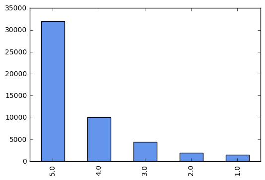
Descriptive Statistics
Let’s take a look at the distribution of scores across reviews.
df['overall'].value_counts().plot(kind='bar', color='cornflowerblue')
<matplotlib.axes._subplots.AxesSubplot at 0x113e6b610>
Naive Bayes
Naive Bayes, in short, uses Bayes rule to find the most likely class for each document. In order to do this it makes a couple of strong assumptions that it is worth being aware of: the position of each word in a document doesn’t matter (bag of words), and feature probabilities are independent given the class (conditional independence). Jurafsky and Manning have a great introduction to Naive Bayes and sentiment analysis. Kevin Markham has slides and accompanying talk that give an introduction to Naive Bayes in scikit-learn.
First, drop observations containg NaN in review or star rating.
print len(df)
df = df[df['reviewText'].notnull()]
print len(df)
df = df[df['overall'].notnull()]
print len(df)
50000
49973
49973
Split into test and training data.
X_train, X_test, y_train, y_test = train_test_split(df['reviewText'],
                                                   df['overall'],
                                                   test_size=.2, random_state=1)
I am going to represent each review as a bag of words, that is, a count of how many times each word appears in a document. Therefore, convert the collection of training reviews into a collection of token counts (a document term matrix).
# instantiate the vectorizer
vect = CountVectorizer()

# tokenize train and test text data
X_train_dtm = vect.fit_transform(X_train)
print "number words in training corpus:", len(vect.get_feature_names())
X_test_dtm = vect.transform(X_test)
number words in training corpus: 36897
Instantiate and train a multinomial naive Bayes model.
nb = MultinomialNB()
%time nb.fit(X_train_dtm, y_train)
CPU times: user 85.8 ms, sys: 17.2 ms, total: 103 ms
Wall time: 111 ms


MultinomialNB(alpha=1.0, class_prior=None, fit_prior=True)
Evaluate the model.
# make class predictions
y_pred = nb.predict(X_test_dtm)

# calculate accuracy, precision, recall, and F-measure of class predictions
def eval_predictions(y_test, y_pred):
    print 'accuracy:', metrics.accuracy_score(y_test, y_pred)
    print 'precision:', metrics.precision_score(y_test, y_pred, average='weighted')
    print 'recall:', metrics.recall_score(y_test, y_pred, average='weighted')
    print 'F-measure:', metrics.f1_score(y_test, y_pred, average='weighted')
eval_predictions(y_test, y_pred)
accuracy: 0.656828414207
precision: 0.604801374748
recall: 0.656828414207
F-measure: 0.615787875508
Take a look at examples where the model is getting it wrong.
# print message text for the first 3 false positives
print 'False positives:'
print
for x in X_test[y_test < y_pred][:2]:
    print x
    print

# print message text for the first 3 false negatives
print 'False negatives:'
print
for x in X_test[y_test > y_pred][:2]:
    print x[:500]
    print
False positives:

My son loves his Elmo, but I have a couple of gripes.  The hard eyes are annoying - he bangs Elmo on his crib bars and I'm nervous he'll crack the eyes one day.  Fabric would have been much nicer.  Also, Elmo's mouth does not open wide like in the picture.  He's got more of a half open mouth.  Other than that, he's squishy and my son likes him, so in that regard, it's a winner.

My children really enjoyed this toy but I really didn't think it was all that great. The only thing they enjoyed about it was the ball. They threw it around a lot.I couldn't get the animals to stand up right, EVER. It is not educational besides the pins are animals. Since the pins don't stand up though the kids don't really pay attention to them.I ended up giving this toy away to someone who had a baby. I thought maybe it would be better for a baby who is learning how to hold things since the game part just doesn't work.

False negatives:

ASSEMBLY: It comes in pieces (the top part with the picture on it, the two half oval pieces that screw to the bottom, and the dowel that runs between the two half ovals) with six screws. Assembly was smooth, with all the pre-drilled spots lining up, but I highly recommend a drill or electric screwdriver. I tried to be lazy at first and just use a screwdriver I had without reach instead of going out to our shed to get the drill, and I gave up. Granted, I could have persevered by hand but it would

This puzzle is amazing. Great quality! My 4 year old LOVES it and it is one of his favorite toys he got for Christmas this year! He was immediately drawn to it and has played with it multiple times so far. He is fascinated by getting to see the inner parts of his body. However my husband pointed out an interesting point. It goes from surface layer (clothes) to deeper and deeper levels (skin, muscle, internal organs and skeleton) However, the skeleton (rib cage for example) protects the internal
Improving Preprocessing
Tokenization is usually accompanied by other preprocessing steps, such as:
- Make all words lowercase
- Remove punctuation
- Tokenize: divide string into a list of substrings.
- Remove words not containing letters
- Remove words containing numbers
- Remove stopwords: stopwords are a list of high frequency words like, the, to, and also.
- Lemmatize: reduces the dimension of the data by aggregating words that either are the same root or have the same meaning.
Let’s try including some of these steps and see if it improves our model.
import string
import nltk
from nltk.stem import WordNetLemmatizer

def no_punctuation_unicode(text):
    '''.translate only takes str. Therefore, to use .translate in the
    tokenizer in TfidfVectorizer I need to write a function that converts
    unicode -> string, applies .translate, and then converts it back'''
    str_text = str(text)
    no_punctuation = str_text.translate(None, string.punctuation)
    unicode_text = no_punctuation.decode('utf-8')
    return unicode_text

def hasNumbers(inputString):
    return any(char.isdigit() for char in inputString)

stoplist = [word.decode('utf-8') for word in nltk.corpus.stopwords.words('english')]

wnl = WordNetLemmatizer()

def prep_review(review):
    lower_case = review.lower()
    no_punct = no_punctuation_unicode(lower_case)
    tokens = nltk.word_tokenize(no_punct)    # weird to tokenize within the vectorizer,
    # but not sure how else to apply functions to each token
    has_letters = [t for t in tokens if re.search('[a-zA-Z]',t)]
    drop_numbers  = [t for t in has_letters if not hasNumbers(t)]
    drop_stops = [t for t in drop_numbers if not t in stoplist]
    lemmed = [wnl.lemmatize(word) for word in drop_stops]
    return lemmed

# tokenize train and test text data
vect = CountVectorizer(tokenizer=prep_review)
X_train_dtm = vect.fit_transform(X_train)
X_test_dtm = vect.transform(X_test)
# instantiate and train model
nb = MultinomialNB()
%time nb.fit(X_train_dtm, y_train)

# evaluate model
y_pred = nb.predict(X_test_dtm)
eval_predictions(y_test, y_pred)
CPU times: user 76.6 ms, sys: 17.6 ms, total: 94.2 ms
Wall time: 138 ms
accuracy: 0.647823911956
precision: 0.563206576672
recall: 0.647823911956
F-measure: 0.564786319837
The extra preprocessing has little effect. In fact, our original approach did slightly better. But can we improve with a different algorithm?
Support Vector Machines
I will also try classifying the reviews using SVMs, which perform classification by constructing hyperplanes to separate different classes. In constructing the hyperplanes, SVMs try firstly to classify observations correctly, and subject to this constraint seek to maximize the margin (the distance between the hyperplane and the nearest point).
I start by creating a TF-IDF matrix. Rather than just measuring the number of times a word appears in a document, as we did above, we now multiply this by the inverse document frequency (the inverse of the number of documents the words appears in). Thus, a words TF-IDF is a measure of relevance. As above, I will initially use limited preprocessing.
tfidf_vectorizer_1 = TfidfVectorizer(min_df=5, max_df=0.8)
tfidf_train_1 = tfidf_vectorizer_1.fit_transform(X_train)
tfidf_test_1 = tfidf_vectorizer_1.transform(X_test)
SVM is a classifier built on giving us linear separation. Kernels are the main technique for adapting SVMs to develop non-linear classifiers, by taking a low-dimensional input space and mapping it to a higher dimensional space. Let’s try SVM with both a linear kernel and an rbf (Gaussian) kernel that maps the features to a higher dimensional space.
# instantiate and train model, kernel=rbf
svm_rbf = svm.SVC(random_state=12345)
%time svm_rbf.fit(tfidf_train_1, y_train)

# evaulate model
y_pred_1 = svm_rbf.predict(tfidf_test_1)
eval_predictions(y_test, y_pred_1)
CPU times: user 16min 18s, sys: 7.27 s, total: 16min 26s
Wall time: 17min 36s
accuracy: 0.63871935968
precision: 0.40796242043
recall: 0.63871935968
F-measure: 0.497903949227
# instantiate and train model, kernel=linear
svm_rbf = svm.SVC(kernel='linear', random_state=12345)
%time svm_rbf.fit(tfidf_train_1, y_train)

# evaulate model
y_pred_1 = svm_rbf.predict(tfidf_test_1)
eval_predictions(y_test, y_pred_1)
CPU times: user 21min 41s, sys: 14.9 s, total: 21min 56s
Wall time: 27min 44s
accuracy: 0.692146073037
precision: 0.642945272553
recall: 0.692146073037
F-measure: 0.649422858215
Now let’s try with the more extensive preprocessing that we used above.
tfidf_vectorizer_2 = TfidfVectorizer(tokenizer=prep_review, min_df=5, max_df=0.8)
tfidf_train_2 = tfidf_vectorizer_2.fit_transform(X_train)
tfidf_test_2 = tfidf_vectorizer_2.transform(X_test)

# kernel=rbf
print 'kernel=rbf'
svm_rbf = svm.SVC(random_state=1)
%time svm_rbf.fit(tfidf_train_2, y_train)
y_pred_2 = svm_rbf.predict(tfidf_test_2)
eval_predictions(y_test, y_pred_2)
print

print 'kernel=linear'
svm_rbf = svm.SVC(kernel='linear', random_state=1)
%time svm_rbf.fit(tfidf_train_2, y_train)
y_pred_2 = svm_rbf.predict(tfidf_test_2)
eval_predictions(y_test, y_pred_2)
kernel=rbf
CPU times: user 10min 35s, sys: 4.51 s, total: 10min 40s
Wall time: 11min 17s
accuracy: 0.63871935968
precision: 0.40796242043
recall: 0.63871935968
F-measure: 0.497903949227

kernel=linear
CPU times: user 14min 44s, sys: 4.71 s, total: 14min 49s
Wall time: 14min 52s
accuracy: 0.681740870435
precision: 0.622991495468
recall: 0.681740870435
F-measure: 0.628936808344
It is suprising that with an rbf kernel we get exactly the same performance with and without the extra preprocessing steps. I have recoded the variables to ensure I’m not accidentally repeating anything. Let’s also print the two vectorizers to check that they are in fact different.
compare_tokens = pd.DataFrame(
    {'unprocessed': tfidf_vectorizer_1.get_feature_names()[:10],
     'preprocessed': tfidf_vectorizer_2.get_feature_names()[:10],
    })
compare_tokens
| preprocessed | unprocessed | |
|---|---|---|
| 0 | aa | 00 |
| 1 | aaa | 000 |
| 2 | ab | 01 |
| 3 | aback | 03 |
| 4 | abacus | 04 |
| 5 | abandon | 07 |
| 6 | abandoned | 08 |
| 7 | abby | 09 |
| 8 | abc | 10 |
| 9 | ability | 100 |
We see that the linear kernel performs best across all predictive measures, and that we actually get slightly better performance without preprocessing. Linear kernels often perform well with text classification because when there are a lot of features, mapping the data to a higher dimensional space does little to improve performance.
Conclusions
The most striking findings here are that it preprocessing makes little difference to the performance of our algorithms and that both naive Bayes and SVMs perform similarly to one another. The latter finding, in particular, is a surprise. Whilst previous research by Banko and Brill has shown that classifiers perform similarly to one another on extremely large corpora, I was not expecting such similar results with our relatively small sample.
If I have time to pursue this project further, there are a number of steps I would like to take:
- explore how unusual it is to have these different models and classifiers perform so similarly, and triple-check that there is no issue with my code
- improve my classifiers, starting by looking at examples that are misclassified
- experiment with other classifiers
- run my models with a larger dataset, ideally, with 142.8 million reviews in McAuley’s full dataset