Can Article Titles Predict Shares?

In this project, I explore whether the content of article titles from the Daily Mail Online can help to predict the number of comments or shares that those articles receive.

My original plan was to focus on the article titles of sponsored content, in order to help sponsors design effective content. However, I found insufficient sponsored items to make this a viable strategy. Considering articles more generally nonetheless presents an interesting challenge, and could be of use to subeditors or others seeking to generate share or reading engagement.

A more detailed discussion of the methods used and complete replication code is available on my GitHub.

Data Collection

I scraped 54,978 articles from the website using Scrapy on an EC2 m4.xlarge instance. For each article, I collected the title, date of publication, category (a label assigned by the website), author, and sponsor (if applicable).

I had originally intended to scrape substantially more websites. However, I found that after scraping several tens of thousands of websites the spider would return a 418 error for all articles, and would continue to do so if I restarted the scraper. I was cautious about continuing as I couldn’t find any clear terms of service. But it would be interesting in future to look into any terms in more detail and to explore tweaking my scraper to try and avoid this issue (for example, perhaps by reducing the number of concurrent requests to the site).

Load Packages and Data

import pandas as pd
import numpy as np
import nltk
import string
import re
import sys
import time
import matplotlib.pyplot as plt

from nltk.stem.snowball import SnowballStemmer

from sklearn.feature_extraction.text import TfidfVectorizer
from sklearn.preprocessing import normalize
from sklearn.cross_validation import train_test_split, cross_val_score
from sklearn.linear_model import LassoLarsCV
from sklearn.metrics import mean_squared_error, mean_absolute_error, pairwise_distances
from sklearn.cluster import KMeans

from xgboost import XGBRegressor
from skopt import gp_minimize
from skopt.plots import plot_convergence

%matplotlib inline

df = pd.read_csv('dm_dat.csv')

# Drop obs with null value in title or pub_time
df = df[df['title'].notnull()]
df = df[df['pub_time'].notnull()]

# Reset index - much quicker to do it here than once I've made tf-idf matrix
df = df.reset_index()

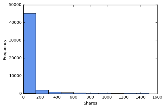
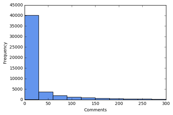
Let’s explore the distributions of shares and comments, and drop outliers.

print 'No shares:', sum(df['shares']==0)*100/float(len(df))
print 'No comments:', sum(df['comments']==0)*100/float(len(df))

print '>1500 shares:', sum(df['shares']>1500)*100/float(len(df))
print '>300 comments:', sum(df['comments']>300)*100/float(len(df))
print '>1500 shares or >300 comments:',sum((df['shares']>1500) | (df['comments']>300))*100/float(len(df))
df = df[(df['shares']<=1500) & (df['comments']<=300)]
df = df.reset_index()

No shares: 57.3339642903
No comments: 52.6764100977
>1500 shares: 5.88792020822
>300 comments: 5.03248821506
>1500 shares or >300 comments: 8.89103252462

plt.hist(df['shares'].tolist(), color='cornflowerblue')
plt.xlabel("Shares")
plt.ylabel("Frequency")
plt.show()
plt.hist(df['comments'].tolist(), color='cornflowerblue')
plt.xlabel("Comments")
plt.ylabel("Frequency")
plt.show()

png

Preprocess Data

Preprocess Non-Text Features

Create dummy variables for key categories.

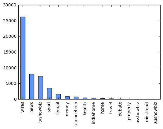
df.category.value_counts().plot(kind='bar', color='cornflowerblue')
pop_cats = ['wires', 'news', 'tvshowbiz', 'sport', 'femail']
for c in pop_cats:
    df['cat_' + c] = 0
    df.loc[df.category==c, 'cat_' + c] = 1

png

Preprocess Text

I need to convert the data from the titles into numerical features. To do this, I will create a TF-IDF matrix. In the process, I will in the following order (although note that there are multiple ways in which these operations could be combined):

Remove all non-ASCII characters: eg. \xe2\x80\x98
Make all words lowercase
Remove punctuation
Tokenize: divide string into a list of substrings.
Remove words not containing letters
Remove words containing numbers
Remove stopwords: stopwords are a list of high frequency words like, the, to, and also.
Stem: take the root of each word.
Remove short words: that is, of 3 characters or less.

I will carry out all but the first of these steps in the process of creating a TF-IDF matrix, below. But we need to prepare the functions beforehand.

def no_punctuation_unicode(text):
    '''.translate only takes str, whereas TfidfVectorizer only takes unicode.
    Therefore, to use .translate in the tokenizer in TfidfVectorizer I need to
    write a function that converts unicode -> string, applies .translate,
    and then converts it back'''
    str_text = str(text)
    no_punctuation = str_text.translate(None, string.punctuation)
    unicode_text = no_punctuation.decode('utf-8')
    return unicode_text

def hasNumbers(inputString):
    return any(char.isdigit() for char in inputString)

def prep_blurb(text):
    lowers = text.lower()
    no_punct = no_punctuation_unicode(lowers)
    tokens = nltk.word_tokenize(no_punct)
    has_letters = [t for t in tokens if re.search('[a-zA-Z]',t)]
    no_numbers  = [t for t in has_letters if not hasNumbers(t)]
    drop_stops = [w for w in no_numbers if not w in stoplist] 
    stems = [stemmer.stem(t) for t in drop_stops]
    drop_short = [s for s in stems if len(s)>2]
    return drop_short

I next extract a matrix of TF-IDF (term frequency-inverse document frequency) features. The tf-idf weight of a term in a document is the product of its tf (term frequency) weight and its idf (inverse document frequency) weight. This is generally given by the formula:

$w_{t,d} = (1 + logtf_{t,d}) \times log_{10}(\frac{N}{df_t})$

Where the term frequency $ tf_{t,d} $ of term t in document d is defined as the number of times that t occurs in d, the document frequency $ df_t $ is he number of documents that contain t, and N is the number of documents. The computation of tf-idfs in scikit-learn is in fact slightly different from the standard textbook notation, but we can ignore that here.

The tf-idf weight (of a term in a document) thus increases with the number of times a term occurs in a document, and also increases with the rarity of the term in the collection.

I will specify some key parameters I define in TfidfVectorizer: ignore words that appear in more than .8 of documents (max_df), ignore words that occur in less than .2 of the documents (min_idf), and use L2 normalization following an scikit-learn example that I draw on later in my Lasso analysis. (I originally tried standardizing the dense dataframe I created from the sparse matrix such that every predictor would have mean=0 and sd=1, following a different Lasso example on Coursera, but this was taking a long time to run.)

# Get list of titles
tlist = df['title'].tolist()

##Remove all non-ASCII characters from titles
new_list = []
for t in tlist:
    new_list.append(t.decode('utf8').encode('ascii', errors='ignore'))
tlist = new_list
    
# Convert items in alist, as TfidfVectorizer only takes unicode
tlist = [t.decode('utf-8') for t in tlist]

# Stopwords must also be in unicode to work with TfidfVectorizer
stoplist = [word.decode('utf-8') for word in nltk.corpus.stopwords.words('english')] 

# Create stemmer
stemmer = SnowballStemmer("english")

# Don't use stop_words argument to TfidfVectorizer as delt with in prep_blurb
tfidf_vectorizer = TfidfVectorizer(tokenizer=prep_blurb, min_df=0.01, norm='l2')
%time tf_idf = tfidf_vectorizer.fit_transform(tlist)

print 'Length initial list:', len(tlist)
print 'tf_idf.shape:', tf_idf.shape
print 'type(tf_idf):', type(tf_idf)

list_of_words = tfidf_vectorizer.get_feature_names()
print 'List of words:', list_of_words[:50]

CPU times: user 1min 1s, sys: 565 ms, total: 1min 2s
Wall time: 1min 6s
Length initial list: 50058
tf_idf.shape: (50058, 104)
type(tf_idf): <class 'scipy.sparse.csr.csr_matrix'>
List of words: [u'ahead', u'arrest', u'attack', u'babi', u'back', u'ban', u'bank', u'boss', u'call', u'car', u'celebr', u'championship', u'charg', u'china', u'citi', u'claim', u'could', u'court', u'cup', u'cut', u'daughter', u'day', u'dead', u'deal', u'death', u'die', u'dress', u'end', u'england', u'face', u'famili', u'fan', u'fashion', u'fight', u'fire', u'first', u'forc', u'former', u'get', u'girl', u'give', u'head', u'help', u'high', u'hit', u'home', u'hous', u'husband', u'kill', u'latest']

Trying different values of min_df df and max_df it becomes clear that the vast majority of words appear in less than 1 percent of documents, while very few words appear in a high proportion of documents. I choose to ignore all words that appear in less than 1 percent of documents.

Extracting tf-idf features, above, gives us a weight matrix between terms and documents. Each document is represented by a row of the matrix, which is a real valued vector, and each term by a column. This will be a sparse matrix, that is, a matrix in which most of the elements are zero.

scikit-learn’s TfidfVectorizer returns a matrix in scipy.sparse.csr format. Printing this matrix shows the nonzero values of the matrix in the (row, col) format.

print 'tf_idf[:2,]:', tf_idf[:2,]

tf_idf[:2,]:   (0, 91)	0.73451170983
  (0, 74)	0.678596012457
  (1, 75)	1.0

In order to include the features from my TF-IDF matrix in my regression model, I need to convert my scipy sparse matrix to a regular dataframe.

df_tfidf = pd.DataFrame(tf_idf.todense())
df_tfidf.columns = list_of_words

I next need to attach my tf-idf matrix dataframe to the other predictor variables. In Lasso regression, the penalty term is not fair if the predictor variables are not on the same scale, as this would mean that not all of the predictors get the same penalty. I normalized the variables in my tf-idf matrix already, and I now need to normalize the non-text variables (I originally tried standardizing, but this was extremely slow - see above discussion of parameters in TfidfVectorizer).

df_notext = df[['pub_days', 'pub_dayofweek', 'pub_sincemid', 'sponsored_dummy', 
                 'cat_wires', 'cat_news', 'cat_tvshowbiz', 'cat_sport', 'cat_femail']]
df_notext_1 = pd.DataFrame(normalize(df_notext, norm='l2', copy=False, axis=0))  #axis=0 normalizes each column
df_notext_1.columns = df_notext.columns.values
df_notext = df_notext_1
del df_notext_1
print df_notext.head(3)

   pub_days  pub_dayofweek  pub_sincemid  sponsored_dummy  cat_wires  \
     0.0       0.001371      0.003118              0.0   0.006175   
     0.0       0.001371      0.003416              0.0   0.006175   
     0.0       0.001371      0.003190              0.0   0.006175   

   cat_news  cat_tvshowbiz  cat_sport  cat_femail  
     0.0            0.0        0.0         0.0  
     0.0            0.0        0.0         0.0  
     0.0            0.0        0.0         0.0  

In joining my tf-idf dataframe with the other variables, concatenating and merging is extremely slow. The quickest approach seems to be to create an empty column for each variable I want to add, and then fill it with the appropriate values.

for c in df_notext.columns.values.tolist():
    df_tfidf[c] = np.nan
    df_tfidf[c] = df_notext[c]

Finally, I need to make sure that I have joined each tf-idf row with the correct values of the other variables (ie. that I have joined all text features to the appropriate observation).

If I try selecting multiple columns from a row of df_tfidf, with a large dataframe it ends up sucking up loads of memory and can grind to a halt (this occurred when I didn’t restrict my tf-idf matrix to words that appeared at least one percent of the time). I believe that problem is that pandas returns copies for most operations. Therefore, I’m better of selecting a row and then examining that.

print df.ix[0]['title']
test_row = df_tfidf.iloc[0]
test_row[test_row>0]

Russia says Trump's efforts on Ukraine better than Obama's - TASS

say              0.678596
trump            0.734512
pub_dayofweek    0.001371
pub_sincemid     0.003118
cat_wires        0.006175
Name: 0, dtype: float64

Lasso Regression

I employ lasso regression, as I have a large number of predictors. Lasso is a shrinkage method for linear regression models that selects the predictors to include. The Lasso imposes a constraint on the sum of the absolute values of the model parameters, where the sum has a specified constant as an upper bound. This constraint causes regression coefficients for some coefficients to shrink towards zero. This is the shrinkage process, which allows for better interpretation of the model and identifies the variables most strongly associated with the outcome of the model.

$\begin{align*} \hat{\beta}^{lasso} &= \arg\min\limits_{\beta}\sum_{i=1}^N\big(y_i - \beta_0 - \sum_{j=1}^px_{ij}\beta_j\big)^2 \\ &s.t. \sum_{j=1}^p|\beta_j| \leq t \end{align*}$

Alternatively, we the model can be written as:

$\hat{\beta}^{lasso} = \Big\{\arg\min\limits_{\beta}\frac{1}{2}\sum_{i=1}^N\big(y_i - \beta_0 - \sum_{j=1}^px_{ij}\beta_j\big)^2 + \lambda\sum_{j=1}^p|\beta_j|\Big\}$

Below, we will use cross-validation to choose the penalty parameter, $ \lambda $. I developed the code below from a scikit-learn example and a Coursera example.

Decide whether to look at shares or comments as outcome. Here I will report the results for shares, but the results for comments are similar.

y = 'shares'
# y = 'comments'

Split the data into a training and test set. (With a larger dataframe, train_test_split makes the memory usage blow up.)

pred_train, pred_test, tar_train, tar_test = train_test_split(df_tfidf.as_matrix(), df[y].as_matrix(),
                                                              test_size=.2, random_state=123)

Specify the lasso regression model. I will use least angle regression (LAR) algorithm to fit the model, and will use cross-validation to select the value of the penalty parameter. Note the scikit-learn calls this penalty parameter $ \alpha $, but the more conventional term is $ \lambda $.

t1 = time.time()
model=LassoLarsCV(cv=10, precompute=False).fit(pred_train, tar_train)
t_lasso_lars_cv = time.time() - t1
print 'train time (seconds):', t_lasso_lars_cv

train time (seconds): 110.333168983

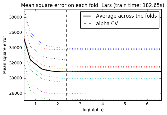
Plot mean square error for each fold.

m_log_alphas = -np.log10(model.cv_alphas_)

plt.figure()
plt.plot(m_log_alphas, model.cv_mse_path_, ':')
plt.plot(m_log_alphas, model.cv_mse_path_.mean(axis=-1), 'k',
         label='Average across the folds', linewidth=2)
plt.axvline(-np.log10(model.alpha_), linestyle='--', color='k',
            label='alpha CV')
plt.legend()

plt.xlabel('-log(alpha)')
plt.ylabel('Mean square error')
plt.title('Mean square error on each fold: Lars (train time: %.2fs)'
          % t_lasso_lars_cv)
plt.axis('tight')
plt.show()

png

Print variable names and regression coefficients.

import operator
coefs = dict(zip(df_tfidf.columns, model.coef_))
coefs = { k:v for k, v in coefs.items() if v!=0 }
print 'Initial number coefs:', df_tfidf.shape[1]
print 'Coefs after fitting model:', len(coefs)
#sorted_coefs_abs = sorted(coefs.items(), key=lambda x:-abs(x[1]))
#sorted_coefs_abs
sorted_coefs = sorted(coefs.items(), key=lambda x:-x[1])
sorted_coefs[:10]

Initial number coefs: 113
Coefs after fitting model: 61





[('cat_news', 6457.1089767405892),
 ('cat_sport', 2338.9548679840141),
 ('cat_femail', 2194.3944872910138),
 ('pub_dayofweek', 674.05328166277548),
 (u'fan', 67.344754789220843),
 (u'mother', 42.871103821600506),
 (u'result', 30.39223099714831),
 (u'die', 28.563209732589247),
 (u'could', 25.716163788410302),
 (u'leagu', 18.913882332635978)]

sorted_coefs[-10:]

[(u'fashion', -12.176155312845649),
 (u'nation', -15.435111782993314),
 (u'husband', -18.05404733809252),
 (u'man', -20.018031968860008),
 (u'car', -28.865403158590983),
 (u'championship', -32.505194129960678),
 (u'england', -61.764827038359272),
 ('pub_days', -265.29318651590592),
 ('pub_sincemid', -1006.3057846628965),
 ('cat_wires', -13891.352753144545)]

How does model do on test data?

def print_errors(model, pred_train, pred_test, tar_train, tar_test):
    # MSE from training and test data
    train_error = mean_squared_error(tar_train, model.predict(pred_train))
    test_error = mean_squared_error(tar_test, model.predict(pred_test))
    print ('training data MSE')
    print(train_error)
    print ('test data MSE')
    print(test_error)
    print

    # MAE from training and test data
    train_error = mean_absolute_error(tar_train, model.predict(pred_train))
    test_error = mean_absolute_error(tar_test, model.predict(pred_test))
    print ('training data MAE')
    print(train_error)
    print ('test data MAE')
    print(test_error)
print_errors(model, pred_train, pred_test, tar_train, tar_test)

training data MSE
30705.4470647
test data MSE
33591.0307443

training data MAE
76.7396327498
test data MAE
79.9628524015

How does this compare to fitting model without text variables?

pred_train, pred_test, tar_train, tar_test = train_test_split(df_notext.as_matrix(), df[y].as_matrix(),
                                                              test_size=.2, random_state=123)

t1 = time.time()
model=LassoLarsCV(cv=20, precompute=False).fit(pred_train, tar_train)
t_lasso_lars_cv = time.time() - t1
print 'trains time (seconds):', t_lasso_lars_cv
print

# Number of coefs after fitting model
coefs = dict(zip(df_notext.columns, model.coef_))
print 'Initial number coefs:', df_notext.shape[1]
print 'Coefs after fitting model:', len(coefs)
print

# MSE and MAE
print_errors(model, pred_train, pred_test, tar_train, tar_test)

trains time (seconds): 2.42720413208

Initial number coefs: 9
Coefs after fitting model: 9

training data MSE
30891.4842252
test data MSE
33684.8088984

training data MAE
76.1813939733
test data MAE
79.182473179

This is rather disappointing. Including text features does not improve the predictive power of our model. This likely results, at least in part, from the fact that such a high proportion of words occur in less than 1 percent of the document titles.

Create Features Using K-Means

Previous research has found that clustering at the preprocessing stage can help to reduce predictive error; for example, Trivedi, Pardos, and Heffernan (2015). If this worked in this context, it would have the added advantage of allowing us to more meaningfully interpret our model; for example, we might be able to say that articles discussing soccer victories are particularly widely shared.

I will use k-means to cluster articles at the pre-processing stage, and then include these clusters as predictors in a regression model. Starting with k cluster centers, k-means identifies which points are nearest to each cluster center. It then chooses new cluster centers by minimizing the total quadratic distance of each cluster center to its points. Then it repeats this process, starting with these new cluster centers.

My dataframe is already to some extent grouped by topic according to the category variable. I will use k-means clustering for only the two largest of these groups: news and wires. I therefore need to attach an id variable to my dataframe so that I don’t loose track of these observations, and then take only the news and wires stories. Note that with a very big dataset (eg. if I am less aggressive in restricting the number of features) non of the following code is going to work absent a huge amount of RAM.

df_tfidf['article_id'] = np.nan
df_tfidf['article_id'] = df['article_id']

I next need to drop non-text variables from dataframe I will use for clustering, as I only want to cluster by text features. Also drop the id variable, but keep this vector for later.

df_1 = df_tfidf[(df_tfidf['cat_news']>0) | (df_tfidf['cat_wires']>0)]
df_1 = df_1.drop(df_notext.columns.values.tolist(), axis=1)  
df_1_id = df_1['article_id']
df_1.drop('article_id', axis=1, inplace=True)
df_1.columns.values

array([u'ahead', u'arrest', u'attack', u'babi', u'back', u'ban', u'bank',
       u'boss', u'call', u'car', u'celebr', u'championship', u'charg',
       u'china', u'citi', u'claim', u'could', u'court', u'cup', u'cut',
       u'daughter', u'day', u'dead', u'deal', u'death', u'die', u'dress',
       u'end', u'england', u'face', u'famili', u'fan', u'fashion',
       u'fight', u'fire', u'first', u'forc', u'former', u'get', u'girl',
       u'give', u'head', u'help', u'high', u'hit', u'home', u'hous',
       u'husband', u'kill', u'latest', u'lead', u'leagu', u'leav', u'life',
       u'like', u'look', u'love', u'make', u'man', u'meet', u'mother',
       u'nation', u'new', u'one', u'open', u'parti', u'plan', u'polic',
       u'presid', u'report', u'result', u'return', u'reveal', u'rise',
       u'say', u'see', u'set', u'share', u'show', u'son', u'south',
       u'stand', u'star', u'state', u'take', u'talk', u'test', u'three',
       u'time', u'top', u'tri', u'trump', u'two', u'use', u'want', u'warn',
       u'week', u'white', u'win', u'woman', u'women', u'work', u'world',
       u'year'], dtype=object)

Then fit model. I tried different numbers of clusters, 6 clusters gives the most meaningful groupings.

n_clusters = 10
kmeans = KMeans(n_clusters=n_clusters, init='k-means++', random_state=0)
%time km = kmeans.fit(df_1)

CPU times: user 11.6 s, sys: 139 ms, total: 11.8 s
Wall time: 6.14 s

I next want to look at some of the text in my different clusters to see if it seems reasonable.

In a good clustering of documents:

Documents in the same cluster should be similar.
Documents from different clusters should be less similar.

To examine the text in my clustering I will:

Fetch 5 nearest neighbors of each centroid from the set of documents assigned to that cluster. I will consider these documents as being representative of the cluster.
Print top 5 words that have highest tf-idf weights in each centroid.

centroids = km.cluster_centers_   # coordinates of cluster centers
cluster_assignment = km.labels_   # label of every data point

for c in xrange(2):    # for c in xrange(n_clusters):
    # Cluster heading
    print('Cluster {0:d}    '.format(c))

    # Print top 5 words with largest TF-IDF weights in the cluster
    idx = centroids[c].argsort()[::-1]
    for i in xrange(5):
        print list_of_words[idx[i]], centroids[c,idx[i]]
    print ('')
    
    # Compute distances from the centroid to all data points in the cluster
    distances = pairwise_distances(tf_idf, [centroids[c]], metric='euclidean').flatten()
    distances[cluster_assignment!=c] = float('inf') # remove non-members from consideration
    nearest_neighbors = distances.argsort() # argsort() returns the indices that would sort an array
    # For 5 nearest neighbors, print the first 250 characters of text
    for i in xrange(5):
        print tlist[nearest_neighbors[i]][:250]
        print ('')
    print('==========================================================')

Cluster 0    
new 0.676215639123
south 0.0329973543237
say 0.0268965803513
deal 0.0241164035692
home 0.0191492984279

PSA unveils new DS7 Crossback sport utility vehicle

Katy Perry rocks vibrant pink suit in promo shots for her new single... after admitting she has 'given up' caring what people think about her style

Kristen Stewart jets out of LA after creating a real buzz with her new shaved hairdo

The Talented Mr Damon: Boston native Matt will narrate a new documentary about the marathon bombing in his hometown

European rights official denounces new Hungarian asylum law

==========================================================
Cluster 1    
win 0.0212595767793
china 0.019911651449
polic 0.0199069152434
top 0.0144398629067
back 0.014095267931

Hoges: The Paul Hogan Story rates behind music biopics INXS and Molly with 1.32M viewers

Fraudster posed as Nickelback's drummer in a bid to swindle $25,000 worth of high-end microphones

Ex-deputy accused of sexually assaulting female inmates

Turkey's treatment of journalist damaging German-Turkish ties-minister

Judge tosses part of ex-University of Kansas rower's lawsuit

==========================================================

These clusterings are far from perfect. For one thing, some clusterings appear to be driven by a word that is in fact not particularly substantively informative, such as “new”, “man”, or “years.” If I explore using k-means further, I could address this by adding customer stopwords. For now, I will include all the categories it gives me, as lasso should end up dropping them if they are not helpful predictors.

An additional concern is that several clusterings appear to be driven by a single word; however, given the relatively small number of words that appear in amore than 1 percent of the article titles, this may be unavoidable. Others are not driven by a single word, but are also not completely consistent in the substantive topics they put together. Thus, the current groupings should be considered a rough-and-ready first cut.

I next create a categorical variable giving the name of the cluster for each observation.

clusters = km.labels_
km_clusters = ['new', 'legal', 'trump', 'man', 'high', 'glob_pol', 
               'killing', 'talks', 'championship', 'years']
for i in range(len(km_clusters)):
    clusters = [km_clusters[i] if x==i else x for x in clusters]
clusters = clusters + [None] * (len(df_notext) - len(clusters))    

Create dataframe with dummy variable for each of the categories and normalize.

df_km = pd.DataFrame({'clusters': clusters})
for c in km_clusters:
    df_km[c] = 0
    df_km.loc[df_km.clusters==c, c] = 1
df_km.drop('clusters', axis=1, inplace=True)
df_km = pd.DataFrame(normalize(df_km, norm='l2', copy=False, axis=0)) 
df_km.columns = km_clusters
print df_km.head(3)

   new     legal     trump  man  high  glob_pol  killing  talks  championship  \
0.0  0.000000  0.022582  0.0   0.0  0.000000      0.0    0.0           0.0   
0.0  0.006365  0.000000  0.0   0.0  0.000000      0.0    0.0           0.0   
0.0  0.000000  0.000000  0.0   0.0  0.024581      0.0    0.0           0.0   

   years  
  0.0  
  0.0  
  0.0  

Merge with df_notext dataframe.

for c in df_notext.columns.values.tolist():
    df_km[c] = np.nan
    df_km[c] = df_notext[c]
print df_km.head(3)

   new     legal     trump  man  high  glob_pol  killing  talks  championship  \
0.0  0.000000  0.022582  0.0   0.0  0.000000      0.0    0.0           0.0   
0.0  0.006365  0.000000  0.0   0.0  0.000000      0.0    0.0           0.0   
0.0  0.000000  0.000000  0.0   0.0  0.024581      0.0    0.0           0.0   

   years  pub_days  pub_dayofweek  pub_sincemid  sponsored_dummy  cat_wires  \
  0.0       0.0       0.001371      0.003118              0.0   0.006175   
  0.0       0.0       0.001371      0.003416              0.0   0.006175   
  0.0       0.0       0.001371      0.003190              0.0   0.006175   

   cat_news  cat_tvshowbiz  cat_sport  cat_femail  
     0.0            0.0        0.0         0.0  
     0.0            0.0        0.0         0.0  
     0.0            0.0        0.0         0.0  

Fit regression model using same approach as above, to ensure comparable.

pred_train, pred_test, tar_train, tar_test = train_test_split(df_km.as_matrix(), df[y].as_matrix(),
                                                              test_size=.2, random_state=123)

t1 = time.time()
model=LassoLarsCV(cv=20, precompute=False).fit(pred_train, tar_train)
t_lasso_lars_cv = time.time() - t1
print 'trains time (seconds):', t_lasso_lars_cv
print

# Number of coefs after fitting model
coefs = dict(zip(df_notext.columns, model.coef_))
print 'Initial number coefs:', df_notext.shape[1]
print 'Coefs after fitting model:', len(coefs)
print

# MSE and MAE
print_errors(model, pred_train, pred_test, tar_train, tar_test)

trains time (seconds): 9.19271206856

Initial number coefs: 9
Coefs after fitting model: 9

training data MSE
30884.8079964
test data MSE
33699.8498576

training data MAE
76.2085491638
test data MAE
79.2159466417

Again, including text data fails to improve the predictive power of the model.

XGBoost

I next try using the XGBoost algorithm, to see if it can make more use of any information in the titles. I initialy go back to using to the dataset that includes both text and non-text features and without features from k-means.

# split into test and training data
X_train, X_test, y_train, y_test = train_test_split(df_tfidf.as_matrix(), df[y].as_matrix(),
                                                    test_size=.2, random_state=123)

# fit the model with defaults
t1 = time.time()
model = XGBRegressor().fit(X_train, y_train)
t = time.time() - t1
print 'train time (seconds):', t

# make and evaluate predictions
print_errors(model, pred_train, pred_test, tar_train, tar_test)

train time (seconds): 16.7377119064
Training data MSE: 29348.6166602
Test data MSE: 33580.7312067
Training data MAE: 74.5390734826
Test data MAE: 79.2257482857

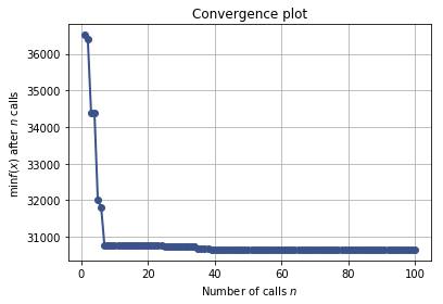
Optimize hyperparameters

# define objective function we want to minimize 
def objective(params):
    max_depth, learning_rate, n_estimators, gamma, min_child_weight, subsample, colsample_bytree = params

    model.set_params(max_depth=max_depth, 
                     learning_rate=learning_rate, 
                     n_estimators=n_estimators, 
                     gamma=gamma,
                     min_child_weight=min_child_weight,
                     subsample=subsample, 
                     colsample_bytree=colsample_bytree)

    return -np.mean(cross_val_score(model, X_train, y_train, cv=5, n_jobs=-1, scoring='neg_mean_squared_error'))

# define bounds of the dimensions of the search space we want to explore
space = [(4, 12),             # max_depth
         (0.01, 0.5),         # learning_rate
         (20, 100),           # n_estimators
         (0, 0.5),            # gamma
         (1, 5),              # min_child_weight
         (0.1, 1),            # subsample
         (0.1, 1)]            # colsample_bytree

model = XGBRegressor()
t1 = time.time()
res_gp = gp_minimize(objective, space, n_calls=100, random_state=0)
t2 = time.time() - t1

print 'Time:', t2
"Best score=%.4f" % res_gp.fun

Time: 2290.87547112
'Best score=30651.1598'

def best_params(res_gp):
    print("""Best parameters:
    - max_depth=%d
    - learning_rate=%.6f
    - n_esimators=%.6f
    - gamma=%.6f
    - min_child_weight=%.6f
    - subsample=%.6f
    - colsample_bytree=%.6f""" % (res_gp.x[0], 
                                  res_gp.x[1], 
                                  res_gp.x[2], 
                                  res_gp.x[3], 
                                  res_gp.x[4], 
                                  res_gp.x[5],
                                  res_gp.x[6]))
best_params(res_gp)

Best parameters:
    - max_depth=4
    - learning_rate=0.122313
    - n_esimators=36.000000
    - gamma=0.000000
    - min_child_weight=1.000000
    - subsample=0.916504
    - colsample_bytree=0.668645

plot_convergence(res_gp)

png

model_opt = XGBRegressor(max_depth=res_gp.x[0], 
                         learning_rate=res_gp.x[1], 
                         n_estimators=res_gp.x[2],
                         gamma=res_gp.x[3], 
                         min_child_weight=res_gp.x[4],
                         subsample=res_gp.x[5],
                         colsample_bytree=res_gp.x[6]).fit(X_train, y_train)
print_errors(model_opt, pred_train, pred_test, tar_train, tar_test)

Training data MSE: 29309.6756115
Test data MSE: 33422.2739789
Training data MAE: 73.4934628747
Test data MAE: 77.9925192076

How does this compare to fitting model without text variables?

X_train, X_test, y_train, y_test = train_test_split(df_notext.as_matrix(), df[y].as_matrix(),
                                                    test_size=.2, random_state=123)

model = XGBRegressor()
res_gp_notext = gp_minimize(objective, space, n_calls=100, random_state=0)

print best_params(res_gp)
plot_convergence(res_gp)

Best parameters:
    - max_depth=4
    - learning_rate=0.122313
    - n_esimators=36.000000
    - gamma=0.000000
    - min_child_weight=1.000000
    - subsample=0.916504
    - colsample_bytree=0.668645

png

model_opt_notext = XGBRegressor(max_depth=res_gp.x[0], 
                         learning_rate=res_gp.x[1], 
                         n_estimators=res_gp.x[2],
                         gamma=res_gp.x[3], 
                         min_child_weight=res_gp.x[4],
                         subsample=res_gp.x[5],
                         colsample_bytree=res_gp.x[6]).fit(X_train, y_train)
print_errors(model_opt_notext, X_train, X_test, y_train, y_test)

Training data MSE: 30246.1536175
Test data MSE: 33340.4866103
Training data MAE: 74.3490005988
Test data MAE: 77.7349067091

XGBoost is a slight improvement on regression. Again, however, including features derived from article headlines does not improve upon a model that includes only non-text features.

Conclusions

In the analyses above, the article titles do not help to predict the number of shares or comments that an article receives any better than using non-text features alone. XGBoost appears to performance slightly better than linear regression.

With more time, I should like to further test this null finding and try to better understand why the text appears to be uninformative. How predictive are article titles in the absence of non-text features? Could I increase the predictive power of my text regression with a better model and/or a larger sample size? What if I also used the text from the article? Does the fact that articles have already been placed into broader categories explain the limited additional predictive power of the article content?

Whilst at present not promising, therefore, the findings in this project present some interesting avenues for future exploration.

Share on

Twitter Facebook Google+ LinkedIn