Predicting NYC 311 Calls
In this mini-project, I try to predict the volumne of calls that NYC’s 311 service will receive in a future time interval.
NYC311 provides access to non-emergency City services and information about City government programs. I count the number of calls received by the service in 10 minute intervals and try to predict the number off calls that will be received in a 10 minute interval one week in the future.
The purpose of this exercise was to gain experience implementing RNNs and get familiar with and interesting dataset. The time interval of 10 minutes was selected to give me sufficient observations to work with, and predicting the number of calls in a single interval one week from today is unlikely to be of much practical. Forecasting call volumes over longer time periods, however, could be valauble in taking steps to meet that demand.
The notebooks for his analysis are available on GitHub.
Data and exploratory analysis
Data on the calls recieved by NYC311 going back to 2010 were downloaded from NYC Open Data. The volume of calls is broken down by agency.
I group the calls into 10 minute intervals and by responding agency, considering the 10 agencies receiving the highest volume of calls and grouping calls to other agencies together.
And initial exploration of the data, grouping instead by daily inervals, reveals a sharp increase in the volume of calls prior to 2016.
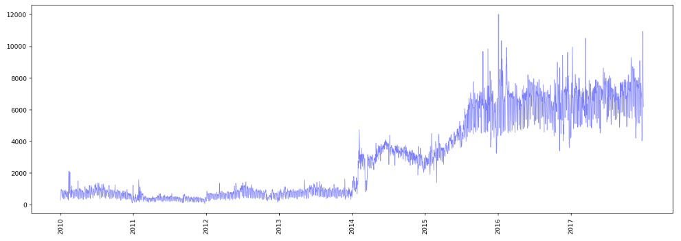
Given this dramatic change in the volume of calls received, I decide to focus on 2016 and 2017 only. I will split this dataset into a training set of the first 65,264 time steps, a validation set of the next 20,000 time steps, and a test tes set of the final 20,000 timesteps.
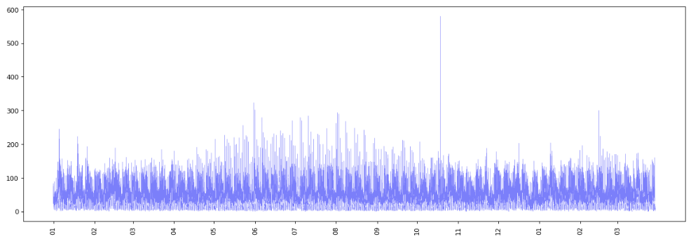
Examing the training set, I see no evidence of heteroskedasticity and no trend in the volume of calls received in 10 minute intervals during this period.
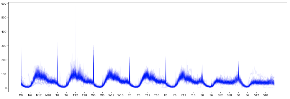
Plotting togheter the 10 minute totals received in each week of the training set we observe a weekly cyclical pattern. I suspect that the spike in calls at midnight is an artefact of the data or my preprocessing of it, rather than a genuine spike at that time, and with more time I would dig into this further.
Calculating a baseline
I would like a simple baseline forecast to compare my models to. I therefore predict the number of calls in one week’s time to be the number of calls in the current period (ie. forecast value is value in same 10 minute period of the previous week), since I am predicting one week in the future and the seasonality of the data appears to be primarily daily. Applying this approach to the validation set results in an MAE of 12.76.
Using RNNs
For each sample (observation) in the training or validation set, I will take loockback time steps (in this case, 6 week’s timesteps) as my inputs for that sample. Note that each time step (each input) has multiple features (the number of calls to each agencies).
I then look forward delay timesteps (in this case, 1 week’s timesteps) for my single target (or prediction): the total number of calls in a 10 minute intervals. This is therefore a many-to-one architecture.
I will fit my model for all observations in the training set and validation set for which I am mble to look both backward and forward a sufficient number of timesteps.
I explored using four different RNN models (building on Francois Chollet (2018) Deep Learning with Python, Chatper 6):
1. A basic model
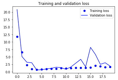
I being my implementing a basic model in which I flattten the data and run it through two dense layers. The validation loss (MAE) falls to around 0.6 after 5 epochs, then increases and remains around 1-3.
model = Sequential()
model.add(layers.Flatten(input_shape=(lookback / step, float_data.shape[-1])))
model.add(layers.Dense(32, activation='relu'))
model.add(layers.Dense(1))

model.compile(optimizer=RMSprop(), loss='mae')
history = model.fit_generator(train_gen,
                              steps_per_epoch=steps_per_epoch
                              epochs=20,
                              validation_data=val_gen,
                              validation_steps=val_steps)
2. A first RNN
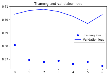
I next fit an RNN with a GRU layer and a dense layer. The MAE of the validation set $\approx 0.4$ after one epoch and the training loss $\approx 0.37$.
model = Sequential()
model.add(layers.GRU(32, input_shape=(None, float_data.shape[-1])))
model.add(layers.Dense(1))

model.compile(optimizer=RMSprop(), loss='mae')
history = model.fit_generator(train_gen,
                              steps_per_epoch=steps_per_epoch,
                              epochs=20,
                              validation_data=val_gen,
                              validation_steps=val_steps)
3. An RNN with recurrent dropout
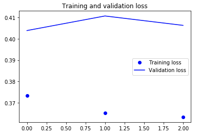
I next change the model to include recurrent dropout, in order to reduce any overfitting. Since the difference in loss between the training and validation set appears small (in substantive terms) I do not expect this to have much effect. Sure enough, the loss is largely unchanged. Unfortunately, it was taking a long time to run so I only ran it for three epochs.
model = Sequential()
model.add(layers.GRU(32,
                     dropout=0.2,
                     recurrent_dropout=0.2,
                     input_shape=(None, float_data.shape[-1])))
model.add(layers.Dense(1))

model.compile(optimizer=RMSprop(), loss='mae')
history = model.fit_generator(train_gen,
                              steps_per_epoch= steps_per_epoch,
                              epochs=7,
                              validation_data=val_gen,
                              validation_steps=val_steps)
4. A dropout-regularized, stacked GRU model
Finally, I try fitting a stacked model. Again, this does not improve the validation MAE.
model = Sequential()
model.add(layers.GRU(32,
                     dropout=0.1,
                     recurrent_dropout=0.5,
                     return_sequences=True,
                     input_shape=(None, float_data.shape[-1])))
model.add(layers.GRU(64, activation='relu',
                     dropout=0.1,
                     recurrent_dropout=0.5))
model.add(layers.Dense(1))
model.compile(optimizer=RMSprop(), loss='mae')
Evaluate on the test set
I evaluate the dropout-regularized model (without stacking) on the test set. Since the performance of all my recurrent models was largely the same it would have made sense to evaluate on the simplist model, however, I didn’t have it saved and wanted to avoid running it again. The MAE on the test set is $\approx 0.39$
Conclusions and next steps
All of the NN models that I tried improved dramatically on my baseline. I was surpised at the extent of the improvement: given how seasonal the data is day-to-day I assumed my baseline would perform quite well. I was also suprised at small the MAE became in relation to the variation in call volumes that we see over time.
I also found that RNN models clearly improved on a more simple baseline model. However, dropout and stacking did not further reduce the loss.
With more time, there are many other avenues I should like to pursue including:
- further tuning the model - for example, adding more layers, or using LSTM layers instead of GRU)
- forecasting multiple steps ahead - this would presumably be of much more practical use than forecasting a single time step, but it somewhat tricky to implement with a RNN
- forecasting for multiple time series - that is, coming up with a separate forecast for each agency’s calls
- comparing the performance of these models to traditional time series models - unfortunately, I found that the data was too large to fit an ARMA model using the astsa package in R